
For simplicity, we can start with an example.
Suppose you have a dataset of 100 apples, and you’ve built a machine learning model to predict whether each apple is “Good” or “Bad” based on certain features like color, size, and texture.
Accuracy:
Accuracy is a measure of how many predictions your model got right overall.
In our example, let’s say your model made predictions for all 100 apples, and 90 of those predictions were correct (i.e., 90 apples were correctly classified as “Good” or “Bad”). The accuracy would be 90%.
Accuracy = (Number of Correct Predictions) / (Total Number of Predictions)
Accuracy = 90 / 100 = 0.90 (or 90%)
So, your model has an accuracy of 90%, meaning it correctly classified 90% of the apples.
Precision:
Precision is a measure of how many of the apples predicted as “Good” by your model were actually “Good.”
Let’s say your model predicted 60 apples as “Good,” and out of those, 55 were actually “Good,” and 5 were “Bad.”
Precision = (Number of True Positives) / (Number of True Positives + Number of False Positives)
Precision = 55 / (55 + 5) = 55 / 60 = 0.917 (or 91.7%)
The precision for “Good” apples is 91.7%. It means that when your model says an apple is “Good,” it is correct about 91.7% of the time.
Recall:
Recall is a measure of how many of the actual “Good” apples were correctly predicted as “Good” by your model.
Out of the 60 actual “Good” apples, let’s say your model correctly predicted 55 as “Good.”
Recall = (Number of True Positives) / (Number of True Positives + Number of False Negatives)
Recall = 55 / (55 + 5) = 55 / 60 = 0.917 (or 91.7%)
The recall for “Good” apples is also 91.7%. It means that your model correctly identified 91.7% of the actual “Good” apples.
In summary
Accuracy tells you how many predictions are correct overall.
Precision tells you how many of the predicted positive cases are actually positive.
Recall tells you how many of the actual positive cases were correctly predicted as positive.
In the case of predicting good and bad apples, you want a balance between high precision and high recall. High precision means your model doesn’t incorrectly label good apples as bad, and high recall means your model doesn’t miss many actual good apples. It’s often a trade-off, and the choice depends on the specific goals of your application.
Contact PravySoft Calicut for machine learning courses
Confusion Matrix
Let’s use the same “Good” and “Bad” apple prediction example to explain a confusion matrix and how it’s represented as a heatmap.
In a confusion matrix, we categorize the model’s predictions and the actual outcomes into four categories:
- True Positives (TP): The model correctly predicted “Good” apples as “Good.”
- True Negatives (TN): The model correctly predicted “Bad” apples as “Bad.”
- False Positives (FP): The model incorrectly predicted “Bad” apples as “Good.”
- False Negatives (FN): The model incorrectly predicted “Good” apples as “Bad.”
Now, let’s say your model made predictions for 100 apples, and here’s the breakdown:
- True Positives (TP): 55 apples were correctly predicted as “Good.”
- True Negatives (TN): 35 apples were correctly predicted as “Bad.”
- False Positives (FP): 5 apples were incorrectly predicted as “Good” when they were actually “Bad.”
- False Negatives (FN): 5 apples were incorrectly predicted as “Bad” when they were actually “Good.”
Your confusion matrix would look like this:
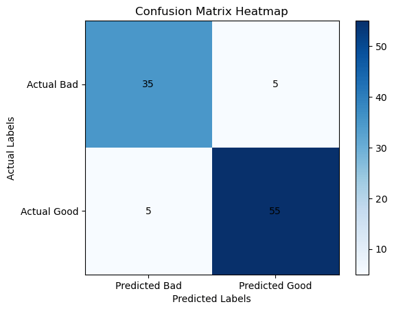
Now, to create a heatmap visualization of this confusion matrix:
- The x-axis represents the predicted labels (Predicted Bad and Predicted Good).
- The y-axis represents the actual labels (Actual Bad and Actual Good).
Each cell in the heatmap represents the count of apples falling into a particular category:
- The top-left cell (Actual Bad, Predicted Bad) contains the True Negatives (TN), which is 35 in our example.
- The top-right cell (Actual Bad, Predicted Good) contains the False Positives (FP), which is 5 in our example.
- The bottom-left cell (Actual Good, Predicted Bad) contains the False Negatives (FN), which is 5 in our example.
- The bottom-right cell (Actual Good, Predicted Good) contains the True Positives (TP), which is 55 in our example.
The heatmap color intensity can be used to visualize the counts. Typically, you would see a dark color (e.g., dark blue) for high counts and a lighter color (e.g., light blue) for low counts.
So, in this example, the heatmap would visually represent the distribution of correct and incorrect predictions for “Good” and “Bad” apples, helping you quickly identify where the model is performing well and where it may need improvement.